It is quite common for the Internet to be visually represented as a cloud, which is perhaps an apt way to think about the Internet given the importance of light and magnetic pulses to its operation. To many people using it, the Internet does seem to lack a concrete physical manifestation beyond our computer and cell phone screens.
But it is important to recognize that our global network of networks does not work using magical water vapor, but is implemented via millions of miles of copper wires and fiber optic cables, as well as via hundreds of thousands or even millions of server computers and probably an equal number of routers, switches, and other networked devices, along with many thousands of air conditioning units and specially constructed server rooms and buildings.
The big picture of all the networking hardware involved in making the Internet work is far beyond our scope here. We should, however, try to provide at least some sense of the hardware that is involved in making the web possible.
From the Computer to the Local Provider
Andrew Blum, in his eye-opening book, Tubes: A Journey to the Center of the Internet, tells the reader that he decided to investigate the question “Where is the Internet” when a hungry squirrel gnawing on some outdoor cable wires disrupted his home connection thereby making him aware of the real-world texture of the Internet.
While you may not have experienced a similar squirrel problem, for many of us, our main experience of the hardware component of the Internet is that which we experience in our homes. While there are many configuration possibilities, Figure 1.18 does provide an approximate simplification of a typical home to local provider setup.
The broadband modem (also called a cable modem or DSL modem) is a bridge between the network hardware outside the house (typically controlled by a phone or cable company) and the network hardware inside the house. These devices are often supplied by the ISP.
 The wireless router is perhaps the most visible manifestation of the Internet in one’s home, in that it is a device we typically need to purchase and install.
Routers are in fact one of the most important and ubiquitous hardware devices that make the Internet work. At its simplest, a router is a hardware device that forwards data packets from one network to another network.
Routers will make use of
Once we leave the confines of our own homes, the hardware of the Internet becomes much murkier.
In Figure 1.18, the various neighborhood broadband cables (which are typically using copper, aluminum, or other metals) are aggregated and connected to fiber optic cable via fiber connection boxes.
Eventually your ISP has to pass on your requests for Internet packets to other networks.
Alternatively, your smaller regional ISP may have transit arrangements with a larger national network (that is, they lease the use of part of their optical fiber network’s bandwidth).
differ in their degree of internal and external interconnectedness.
 Clearly this is an inefficient system, but is a reasonable approximation of the state of the Internet in the late 1990s (and in some regions of the world this is still the case), when almost all Internet traffic went through a few Network Access Points (NAP), most of which were in the United States.
This type of network configuration began to change in the 2000s, as more and more networks began to interconnect with each other using an Internet exchange point (IX or IXP). These IXPs allow different ISPs to peer with one another (that is, interconnect) in a shared facility, thereby improving performance for each partner in
the peer relationship(List of Internet exchange points).
Figure 1.21 illustrates how the configuration shown in Figure 1.20 changes with the use of IXPs.
 As you can see in Figure 1.22, different networks connect not only to other networks within an IXP, but now large websites such as Microsoft and Facebook are also connecting to multiple other networks simultaneously as a way of improving the performance of their sites.
Real IXPs, such as at Palo Alto (PAIX), Amsterdam (AMS-IX), Frankfurt (CE-CIX), and London (LINX), allow many hundreds of networks and companies to interconnect and have throughput of over 1000 gigabits per second. The scale of peering in these IXPs
is way beyond that shown in Figure 1.22 (which shows peering with only five others); companies within these IXPs use large routers from Cisco and Brocade that have hundreds of ports allowing hundreds of simultaneous peering relationships.
In recent years, major web companies have joined the network companies in making use of IXPs.
As shown in Figure 1.23, this sometimes involves mirroring (duplicating) a site’s infrastructure (i.e., web and data servers) in a data center located near the IXP.
For instance, Equinix Ashburn IX in Ashburn, Virginia, is surrounded by several gigantic data centers just across the street from the IXP.
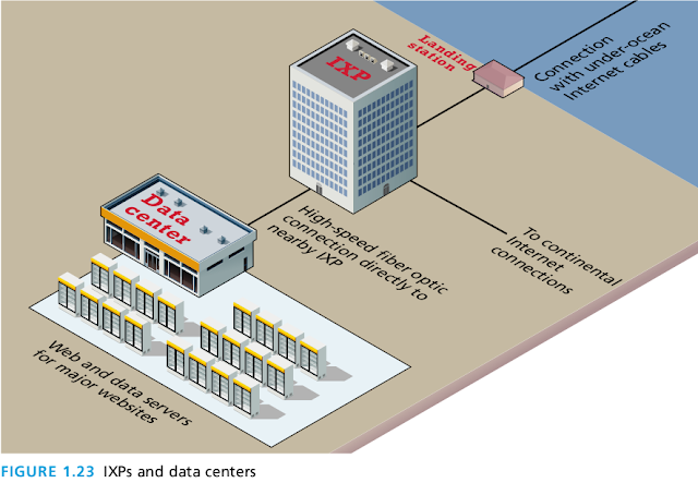
This concrete geography to the digital world encapsulates an arrangement that benefits both the networks and the web companies. The website will have incremental speed enhancements (by reducing the travel distance for these sites) across all the networks it is peered with at the IXP, while the network will have
improved performance for its customers when they visit the most popular websites.
Across the Oceans
Eventually, international Internet communication will need to travel underwater.
The amount of undersea fiber optic cable is quite staggering and is growing yearly.
As can be seen in Figure 1.24, over 250 undersea fiber optic cable systems operated by a variety of different companies span the globe.
 For places not serviced by under sea cable (such as Antarctica, much of the Canadian Arctic islands, and other small islands throughout the world), Internet connectivity is provided by orbiting satellites. It should be noted that satellite links (which have smaller bandwidth in comparison to fiber optic) account for an exceptionally small percentage of oversea Internet communication.
But it is important to recognize that our global network of networks does not work using magical water vapor, but is implemented via millions of miles of copper wires and fiber optic cables, as well as via hundreds of thousands or even millions of server computers and probably an equal number of routers, switches, and other networked devices, along with many thousands of air conditioning units and specially constructed server rooms and buildings.
The big picture of all the networking hardware involved in making the Internet work is far beyond our scope here. We should, however, try to provide at least some sense of the hardware that is involved in making the web possible.
From the Computer to the Local Provider
Andrew Blum, in his eye-opening book, Tubes: A Journey to the Center of the Internet, tells the reader that he decided to investigate the question “Where is the Internet” when a hungry squirrel gnawing on some outdoor cable wires disrupted his home connection thereby making him aware of the real-world texture of the Internet.
While you may not have experienced a similar squirrel problem, for many of us, our main experience of the hardware component of the Internet is that which we experience in our homes. While there are many configuration possibilities, Figure 1.18 does provide an approximate simplification of a typical home to local provider setup.
The broadband modem (also called a cable modem or DSL modem) is a bridge between the network hardware outside the house (typically controlled by a phone or cable company) and the network hardware inside the house. These devices are often supplied by the ISP.

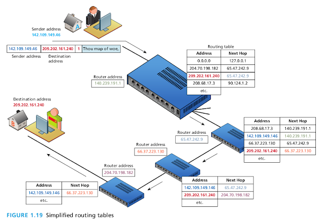
Routers are in fact one of the most important and ubiquitous hardware devices that make the Internet work. At its simplest, a router is a hardware device that forwards data packets from one network to another network.
- When the router receives a data packet, it examines the packet’s destination address and then forwards it to another destination by deciding the best path to send the packets.
- A router uses a routing table to help determine where a packet should be sent. It is a table of connections between target addresses and the node (typically another router) to which the router can deliver the packet.

Routers will make use of
- submasks,
- timestamps,
- distance metrics, and
- routing algorithms
Once we leave the confines of our own homes, the hardware of the Internet becomes much murkier.
In Figure 1.18, the various neighborhood broadband cables (which are typically using copper, aluminum, or other metals) are aggregated and connected to fiber optic cable via fiber connection boxes.
Fiber optic cable (or simply optical fiber) is a glass-based wire that transmits light and has significantly greater bandwidth and speed in comparison to metal wires.In some cities (or large buildings), you may have fiber optic cable going directly into individual buildings; in such a case the fiber junction box will reside in the building.
- These fiber optic cables eventually make their way to an ISP’s head-end, which is a facility that may contain a cable modem termination system (CMTS) or a digital subscriber line access multiplexer (DSLAM) in a DSL-based system.
- This is a special type of very large router that connects and aggregates subscriber connections to the larger Internet.
- These different head-ends may connect directly to the wider Internet,
- or instead be connected to a master head-end, which provides the connection to the rest of the Internet.
Eventually your ISP has to pass on your requests for Internet packets to other networks.
- This intermediate step typically involves one or more regional network hubs.
- Your ISP may have a large national network with optical fiber connecting most of the main cities in the country.
- Some countries have multiple national or regional networks, each with their own optical network.
Alternatively, your smaller regional ISP may have transit arrangements with a larger national network (that is, they lease the use of part of their optical fiber network’s bandwidth).
A general principle in network design is that the fewer the router hops (and thus the more direct the path), the quicker the response.Figure 1.20 illustrates some hypothetical connections between several different networks spread across four countries. As you can see, just like in the real world, the countries in the illustration
differ in their degree of internal and external interconnectedness.
- The networks in Country A are all interconnected, but rely on Network A1 to connect them to the networks in Country B and C.
- Network B1 has many connections to other countries’ networks.
- The networks within Country C and D are not interconnected, and thus rely on connections to international networks in order to transfer information between the two domestic networks. For instance, even though the actual distance between a node in Network C1 and a node in C2 might only be a few miles, those packets might have to travel many hundreds or even thousands of miles between networks A1 and/or B1.

This type of network configuration began to change in the 2000s, as more and more networks began to interconnect with each other using an Internet exchange point (IX or IXP). These IXPs allow different ISPs to peer with one another (that is, interconnect) in a shared facility, thereby improving performance for each partner in
the peer relationship(List of Internet exchange points).
Figure 1.21 illustrates how the configuration shown in Figure 1.20 changes with the use of IXPs.
- As you can see, IXPs provide a way for networks within a country to interconnect. Now networks in Countries C and D no longer need to make hops out of their country for domestic communications.
- Notice as well that for each of the IXPs, there are connections not just with networks within their country, but also with other countries’ networks as well.
- Multiple paths between IXPs provide a powerful way to handle outages and keep packets flowing.
- Another key strength of IXPs is that they provide an easy way for networks to connect to many other networks at a single location.11

Real IXPs, such as at Palo Alto (PAIX), Amsterdam (AMS-IX), Frankfurt (CE-CIX), and London (LINX), allow many hundreds of networks and companies to interconnect and have throughput of over 1000 gigabits per second. The scale of peering in these IXPs
is way beyond that shown in Figure 1.22 (which shows peering with only five others); companies within these IXPs use large routers from Cisco and Brocade that have hundreds of ports allowing hundreds of simultaneous peering relationships.
In recent years, major web companies have joined the network companies in making use of IXPs.
As shown in Figure 1.23, this sometimes involves mirroring (duplicating) a site’s infrastructure (i.e., web and data servers) in a data center located near the IXP.
For instance, Equinix Ashburn IX in Ashburn, Virginia, is surrounded by several gigantic data centers just across the street from the IXP.

This concrete geography to the digital world encapsulates an arrangement that benefits both the networks and the web companies. The website will have incremental speed enhancements (by reducing the travel distance for these sites) across all the networks it is peered with at the IXP, while the network will have
improved performance for its customers when they visit the most popular websites.
Across the Oceans
Eventually, international Internet communication will need to travel underwater.
The amount of undersea fiber optic cable is quite staggering and is growing yearly.
As can be seen in Figure 1.24, over 250 undersea fiber optic cable systems operated by a variety of different companies span the globe.

Resources
- Fundamentals of Web Development by Randy Connolly, Ricardo Hoar
- How Does the Internet Work? - Stanford University
- How does the Internet work?
- Internet Basics - What is the Internet?
- Advanced Networking | Internet2