The concept of a programmable system-on-chip (SoC) started in 1972 with the advent of the unassuming 4-bit TMS1000 microcomputer —the perfect fit for applications such as calculators and microwave ovens that required a device with everything needed to embed "electronic intelligence".
Microcomputers changed the way engineers approached equipment design;
Today’s MCU, just like yesterday’s microcomputer, remains the heart and soul of many systems.
Today, young engineers requested by their superiors to design an analog control system, have an entirely new technique available to them to help them design the system and overcome the “old” problems.
The design technique is this:
Intro
Designers of analog electronic control systems have continually faced the following obstacles in arriving at a satisfactory design:
The alternative new design technique for analog systems is to
A Refresher
Since we deal with the electronic functions and circuits that interface or couple analog-to-digital circuits and systems, or vice versa, a short review is provided so it is clearly understood what analog means and what digital means.
Analog
 An ink pen records the temperature in degrees Fahrenheit and plots it continuously against time on a special graph paper attached to a drum as the drum rotates.
The record of the temperature changes is shown in Figure 1-1b.
 The electrical circuit consists of a potentiometer, basically a resistor connected across a car battery from the positive terminal to the negative terminal, which is grounded. The resistor has a variable tap that is rotated by a float riding on the surface of the liquid inside the gas tank.
A voltmeter reads the voltage from the variable tap to the negative side of the battery (ground) abbreviated as GND (black), 0V, usually connected to the vehicle's metal chassis and body.
The voltmeter indicates the information about the amount of fuel in the gas tank.
An analog of the fuel level is said to be a copy of the fuel level in another form—it is analogous to the original fuel level.
The system shown in Figure 1-3 is a simplified version of the original telegraph system, but it will demonstrate the principle and help to define a digital system.

The electrical circuit (Figure 1-3a) is a battery with a switch in the line at one end and a light bulb at the other.
The two levels—ON and OFF—are most commonly identified as 1(one) and zero (0) in modern binary digital systems, and the 1 and 0 are called binary digits or bits for short.
 To represent larger quantities more bits are added.
For example, a 16-bit code can represent 2^16=65,536 quantities.
Our normal numbering system is a decimal system. Figure 1-5 is a summary showing the characteristics of a decimal and a binary numbering system.
 Note that each system in Figure 1-5 has specific digit positions with specific assigned values to each position. Only eight digits are shown for each system in Figure 1-5.
Example 1. Identifying the Weighted Digit Positions of a Decimal Number
Separate out the weighted digit positions of 6524.
Solution:
6524 = 6 × 10^3 + 5 × 10^2 + 2 × 10^1 + 4 × 10^0
6524 = 6 × 1000 + 5 × 100 + 2 X 10 + 4 × 1
6524 = 6000 + 500 + 20 + 4
Can be identified as 652410 since decimal is a
base 10 system. Normally 10 is omitted since
it is understood.
Example 2. Converting a Decimal Number to a Binary Number
Convert 103 to a binary number.
Solution:
10310 / 2 = 51 with a remainder of 1
51/2 = 25 with a remainder of 1
25/2 = 12 with a remainder of 1
12/2 = 6 with a remainder of 0
6/2 = 3 with a remainder of 0
3/2 = 1 with a remainder of 1
1/2 = 0 with a remainder of 1 (MSB)
10310 = 1100111
Example 3. Determining the Decimal Value of a Binary Number
What decimal value is the binary number 1010111?
Solution:
Solve this the same as Example 1, but use the binary digit weighted position values.
Since this is a 7-bit number:
And since the MSB is a 1, then MSB = 1 × 2^6 = 64
and (next digit) 0 × 2^5 = 0
and (next digit) 1 × 2^4 = 16
and (next digit) 0 × 2^3 = 0
and (next digit) 1 × 2^2 = 4
and (next digit) 1 × 2^1 = 2
and (next digit, LSB) 1 × 2^0 = 1
----------
87
Binary Alphanumeric Quantities
If alphanumeric characters are to be represented, then Figure 1-6, the ASCII table defines the codes that are used.
For example, it is a 7-bit code, and capital M is represented by 1001101. Bit #1 is the LSB and bit #7 is the MSB.
 As shown, upper and lower case alphabet, numbers, symbols, and communication codes are represented.
Accuracy vs. Speed — Analog and Digital
Quantities in nature and in the human world are typically analog. The temperature, pressure, humidity and wind velocity in our environment all change smoothly and continuously, and in many cases, slowly.
Using 12 bits gives four times the accuracy (1 part in 4096, 2^12=4096), and
using 16 bits gives an accuracy of 0.0015%(2^16=65536), or
1 part in 65,536.
 The complete procedure is indicated in Figure 1-7, and the need for analog circuits, digital circuits and the conversion circuits between them is immediately apparent.
Interface Electronics
The system shown in Figure 1-7 shows the major functions needed to couple analog signals to digital systems that
The Basic Functions for Analog-to-Digital Conversion
Sensing the Input Signal
Figure 1-8 separates out the analog-to-digital portion of the Figure 1-7 chain to expand the basic functions in the chain.
Most of nature’s inputs such as temperature, pressure, humidity, wind velocity, speed, flow rate, linear motion or position are not in a form to input them directly to electronic systems.
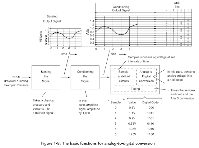 The basic function of the first block is called sensing. The components that sense physical quantities and output electrical signals are called sensors.
The sensor illustrated in Figure 1-8 measures pressure. The output is in millivolts and is an analog of the pressure sensed. An example output plotted against time is shown.
Conditioning the Signal
Conditioning the signal means that some characteristic of the signal is being changed. In Figure 1-8, the block is an amplifier that increases the amplitude of the signal by 1,000 times so that the output signal is now in volts rather than millivolts.
Analog-to-Digital Conversion
In the basic analog-to-digital conversion function, as shown in Figure 1-7, the analog signal must be changed to a digital code so it can be recognized by a digital system that processes the information.
Since the analog signal is changing continuously, a basic subfunction is required. It is called a sample-and-hold function.
For the analog signal shown in the plot of voltage against time and the 4-bit codes given for the indicated analog voltages, identify the analog voltage values at the sample points and the resultant digital
codes and fill in the following table.
 Obviously, one would like to increase the sampling rate to reduce this error.
However, depending on the code conversion time, if the sample rate gets to large, there is not enough time for the conversion to be completed and the conversion function fails.
Other converters may present the codes in a serial string. It depends on the conversion design and the application.
Summary
So far we reviewed
important to have these basic functions in mind as the electronic circuits that perform these functions are the "core business" of our work.__
Microcomputers changed the way engineers approached equipment design;
- for the first time they could reuse proven electronics hardware, needing only to create software specific to the application.
- The result of microcomputer-based designs has been a reduction in both system cost and time-to-market.
Today’s MCU, just like yesterday’s microcomputer, remains the heart and soul of many systems.
- But over time the MCU has placed more emphasis on providing a higher level of integration and control processing and less on sheer computing power.
- The race for embedded computing power has been won by the dedicated digital signal processor (DSP), a widely used invention of the ‘80s that now dominates high-volume, computing-intensive embedded applications such as the cellular telephone. But the design engineer’s most used tool, when it comes to implementing cost effective system integration, remains the MCU. The MCU allows just the right amount of intelligent control for a wide variety of applications.
- Today there are hundreds of MCUs readily available, from low-end 4-bit devices like those found in a simple wristwatch, to high-end 64-bit devices. But the workhorses of the industry are still the versatile 8/16-bit architectures. Choices are available with 8 to 100+ pins and program memory ranging from 1 kb to 64 KB.
- The MCU’s adoption of mixed-signal peripherals is an area that has greatly expanded, recently enabling many new SoC solutions. It is common today to find MCUs with 12-bit analog-to-digital and digital-to-analog converters combined with amplifiers and power management, all on the same chip in the same device. This class of device offers a complete signal-chain on a chip for applications ranging from energy meters to personal medical devices.
- Modern MCUs combine mixed-signal integration with instantly programmable Flash memory and embedded emulation.
- In the hands of a savvy engineer, a unique MCU solution can be developed in just days or weeks compared to what used to take months or years.
- You can find MCUs everywhere you look from the watch on your wrist to the cooking appliances in your home to the car you drive. An estimated 20 million MCUs ship every day(2005), with growth forecast for at least a decade to come. The march of increasing silicon integration will continue offering an even greater variety of available solutions—but it is the engineer’s creativity that will continue to set apart particular system solutions.
- without severe nonlinearity, or
- because the circuits drifted or became unstable with temperature, or
- because the computations using analog signals were quite inaccurate.
Today, young engineers requested by their superiors to design an analog control system, have an entirely new technique available to them to help them design the system and overcome the “old” problems.
The design technique is this:
- sense the analog signals and convert them to electrical signals;
- condition the signals so they are in a range of inputs to assure accurate processing;
- convert the analog signals to digital; make the necessary computations using the very high-speed IC digital processors available with their high accuracy;
- convert the digital signals back to analog signals; and
- output the analog signals to perform the task at hand.
- different types of sensors and their outputs.
- different techniques of conditioning the sensor signals, especially amplifiers and op amps.
- techniques and circuits for analog-to-digital and digital-to-analog conversions, and what a digital processor is and how it works.
- data transmissions and power control
- assembly-language programming, and also
- hands on experience on building a working project.
- ability on choosing a digital processor. We choose to use TI MSP430 microcontroller because of its design, and because it is readily available, it is well supported with design and applications documentation, and it has relatively inexpensive evaluation tools.
Intro
Designers of analog electronic control systems have continually faced the following obstacles in arriving at a satisfactory design:
- Instability and drift due to temperature variations.
- Dynamic range of signals and non-linearity when pressing the limits of the range.
- Inaccuracies of computation when using analog quantities.
- Adequate signal frequency range.
The alternative new design technique for analog systems is to
- sense the analog signal,
- convert it to digital signals,
- use the speed and accuracy of digital circuits to do the computations, and
- convert the resultant digital output back to analog signals.
- First, between analog and digital systems, and
- second, between the external human world and the internal electronics world.
- First, from the human world to the electronics world and back again and,
- in a similar fashion, from the analog systems to digital systems and back again.
- the electronic functions needed, and
- describe how electronic circuits are designed and applied to implement the functions,and
- give examples of the use of the functions in systems.
A Refresher
Since we deal with the electronic functions and circuits that interface or couple analog-to-digital circuits and systems, or vice versa, a short review is provided so it is clearly understood what analog means and what digital means.
Analog
- Analog quantities vary continuously, and
- analog systems represent the analog information using electrical signals that vary smoothly and continuously over a range.

The record of the temperature changes is shown in Figure 1-1b.
Note that the temperature changes smoothly and continuously. There are no abrupt steps or breaks in the data.Another example is the automobile fuel gauge system shown in Figure 1-2.

A voltmeter reads the voltage from the variable tap to the negative side of the battery (ground) abbreviated as GND (black), 0V, usually connected to the vehicle's metal chassis and body.
The voltmeter indicates the information about the amount of fuel in the gas tank.
It represents the fuel level in the tank.The greater the fuel level in the tank the greater the voltage reading on the voltmeter.The voltage is said to be an analog of the fuel level.
An analog of the fuel level is said to be a copy of the fuel level in another form—it is analogous to the original fuel level.
The voltage (fuel level) changes smoothly and continuously so the system is an analog system, but is also an analog system because the system output voltage is a copy of the actual output parameter (fuel level) in another form.Digital
Digital quantities vary in discrete levels.In most cases, the discrete levels are just two values—ON and OFF.
Digital systems carry information using combinations of ON-OFF electrical signals that are usually in the form of codes that represent the information.The telegraph system is an example of a digital system.
The system shown in Figure 1-3 is a simplified version of the original telegraph system, but it will demonstrate the principle and help to define a digital system.

The electrical circuit (Figure 1-3a) is a battery with a switch in the line at one end and a light bulb at the other.
- The person at the switch position is remotely located from the person at the light bulb.
- The information is transmitted from the person at the switch position to the person at the light bulb by coding the information to be sent using the International Morse telegraph code.
- Morse code uses short pulses (dots) and long pulses (dashes) of current to form the code for letters or numbers as shown in Figure 1-3b. As shown in Figure 1-3c, combining the codes of dots and dashes for the letters and numbers into words sends the information.
- The sender keeps the same shorter time interval between letters but a longer time interval between words. This allows the receiver to identify that the code sent is a character in a word or the end of a word itself. The T is one dash (one long current pulse). The H is four short dots (four short current pulses). The R is a dot-dash-dot. And the two Es are a dot each.
- The two states are ON and OFF—current or no current. The person at the light bulb position identifies the code by watching the glow of the light bulb. In the original telegraph, this person listened to a buzzer or “sounder”to identify the code.
- Coded patterns of changes from one state to another as time passes carry the information.
- At any instant of time the signal is either one of two levels. The variations in the signal are always between set discrete levels, but, in addition, a very important component of digital systems is the timing of signals. In many cases, digital signals, either at discrete levels, or changing between discrete levels, must occur precisely at the proper time or the digital system will not work.
- Timing is maintained in digital systems by circuits called system clocks.
This is what identifies a digital signal and the information being processed in a digital system.
The two levels—ON and OFF—are most commonly identified as 1(one) and zero (0) in modern binary digital systems, and the 1 and 0 are called binary digits or bits for short.
Since the system is binary (two levels), the maximum code combinations 2^n depends on the number of bits, n, used to represent the information.For example, if numbers were the only quantities represented, then the codes would look like Figure 1-4, when using a 4-bit code to represent 16 quantities.

For example, a 16-bit code can represent 2^16=65,536 quantities.
The first bit at the right edge of the code is called the least significant bit (LSB). The left-most bit is called the most significant bit (MSB).Binary Numerical Quantities
Our normal numbering system is a decimal system. Figure 1-5 is a summary showing the characteristics of a decimal and a binary numbering system.

- Note that in each system, the LSB is either 100 in the decimal system or 20 in the binary system.
- Each of these has a value of one since any number to the zero power is equal to one.
Example 1. Identifying the Weighted Digit Positions of a Decimal Number
Separate out the weighted digit positions of 6524.
Solution:
6524 = 6 × 10^3 + 5 × 10^2 + 2 × 10^1 + 4 × 10^0
6524 = 6 × 1000 + 5 × 100 + 2 X 10 + 4 × 1
6524 = 6000 + 500 + 20 + 4
Can be identified as 652410 since decimal is a
base 10 system. Normally 10 is omitted since
it is understood.
Example 2. Converting a Decimal Number to a Binary Number
Convert 103 to a binary number.
Solution:
10310 / 2 = 51 with a remainder of 1
51/2 = 25 with a remainder of 1
25/2 = 12 with a remainder of 1
12/2 = 6 with a remainder of 0
6/2 = 3 with a remainder of 0
3/2 = 1 with a remainder of 1
1/2 = 0 with a remainder of 1 (MSB)
10310 = 1100111
Example 3. Determining the Decimal Value of a Binary Number
What decimal value is the binary number 1010111?
Solution:
Solve this the same as Example 1, but use the binary digit weighted position values.
Since this is a 7-bit number:
And since the MSB is a 1, then MSB = 1 × 2^6 = 64
and (next digit) 0 × 2^5 = 0
and (next digit) 1 × 2^4 = 16
and (next digit) 0 × 2^3 = 0
and (next digit) 1 × 2^2 = 4
and (next digit) 1 × 2^1 = 2
and (next digit, LSB) 1 × 2^0 = 1
----------
87
Binary Alphanumeric Quantities
If alphanumeric characters are to be represented, then Figure 1-6, the ASCII table defines the codes that are used.
For example, it is a 7-bit code, and capital M is represented by 1001101. Bit #1 is the LSB and bit #7 is the MSB.

Accuracy vs. Speed — Analog and Digital
Quantities in nature and in the human world are typically analog. The temperature, pressure, humidity and wind velocity in our environment all change smoothly and continuously, and in many cases, slowly.
Instruments that measure analog quantities usually have slow response and less than high accuracy.To maintain an accuracy of 0.1% or 1 part in 1000 is difficult with an analog instrument.
Digital quantities, on the other hand, can be maintained at very high accuracy and measured and manipulated at very high speed.
The accuracy of the digital signal is in direct relationship to the number of bits used to represent the digital quantity.For example, using 10 bits, an accuracy of 1 part in 1024 (2^10=1204) is assured.
Using 12 bits gives four times the accuracy (1 part in 4096, 2^12=4096), and
using 16 bits gives an accuracy of 0.0015%(2^16=65536), or
1 part in 65,536.
And this accuracy can be maintained as digital quantities are manipulated and processed very rapidly, millions of times faster than analog signals.The advent of the integrated circuit has propelled the use of digital systems and digital processing.
The small space required to handle a large number of bits at high speed and high accuracy, at a reasonable price, promotes their use for high-speed calculations.As a result, if analog quantities are required to be processed and manipulated, the new design technique is to
- first convert the analog quantities to digital quantities,
- process them in digital form,
- reconvert the result to analog signals and
- output them to their destination to accomplish a required task.

Interface Electronics
The system shown in Figure 1-7 shows the major functions needed to couple analog signals to digital systems that
- perform calculations,
- manipulate, and
- process the digital signals and
- then return the signals to analog form.
The Basic Functions for Analog-to-Digital Conversion
Sensing the Input Signal
Figure 1-8 separates out the analog-to-digital portion of the Figure 1-7 chain to expand the basic functions in the chain.
Most of nature’s inputs such as temperature, pressure, humidity, wind velocity, speed, flow rate, linear motion or position are not in a form to input them directly to electronic systems.
They must be changed to an electrical quantity—a voltage or a current—in order to interface to electronic circuits.

The sensor illustrated in Figure 1-8 measures pressure. The output is in millivolts and is an analog of the pressure sensed. An example output plotted against time is shown.
Conditioning the Signal
Conditioning the signal means that some characteristic of the signal is being changed. In Figure 1-8, the block is an amplifier that increases the amplitude of the signal by 1,000 times so that the output signal is now in volts rather than millivolts.
The amplification is linear and the output is an exact reproduction of the input, just changed in amplitude.Other signal conditioning circuits may
- reduce the signal level, or
- do a frequency selection (filtering), or
- perform an impedance conversion.
Analog-to-Digital Conversion
In the basic analog-to-digital conversion function, as shown in Figure 1-7, the analog signal must be changed to a digital code so it can be recognized by a digital system that processes the information.
Since the analog signal is changing continuously, a basic subfunction is required. It is called a sample-and-hold function.
- Timing circuits (clocks) set the sample interval and the function takes a sample of the input signal and holds on to it.
- The sample-and-hold value is fed to the analog-to-digital converter that generates a digital code whose value is equivalent to the sample-and-hold value. This is illustrated in Figure 1-8 as the conditioned output signal is sampled at intervals 0, 1, 2, 3, and 4 and converted to the 4-bit codes shown.
- Because the analog signal changes continually, there maybe an error between the true input voltage and the voltage recorded at the next sample.
For the analog signal shown in the plot of voltage against time and the 4-bit codes given for the indicated analog voltages, identify the analog voltage values at the sample points and the resultant digital
codes and fill in the following table.

However, depending on the code conversion time, if the sample rate gets to large, there is not enough time for the conversion to be completed and the conversion function fails.
Thus, there is a compromise in the analog-to-digital converter between the speed of the conversion process and the sampling rate.Output signal accuracy also plays a part. If the output requires more bits to be able to represent the magnitude and the accuracy required, then higher-speed conversion circuits and more of them are going to be required.
Thus, design time, cost, and all the design guidelines enter in.As shown in Figure 1-8, the bits of the digital code are presented all at the same time (in parallel) at each sample point.
Other converters may present the codes in a serial string. It depends on the conversion design and the application.
Summary
So far we reviewed
- analog and digital signals and systems,
- digital codes,
- the decimal and binary number systems, and
- the basic functions required to convert analog signals to digital signals.
important to have these basic functions in mind as the electronic circuits that perform these functions are the "core business" of our work.__
Resources
- Foundations of Analog and Digital Electronic Circuits
- Home » Courses » Electrical Engineering and Computer Science » Circuits and Electronics
- The University Program (
- Electronics I and II
- Analog and Digital Circuits for Electronic Control System Applications
- Fundamentals of Digital Electronics
- Notes on Digital Circuits
- Analog to Digital (ADC) and Digital to Analog (DAC) Converters
- Digital Vs Analog control
- Digital to Analog Converter--DAC (slides)
- Analog-Digital Interface Integrated Circuits (slides)
- Analog-Digital Interface Integrated Circuits
- Digital-to-Analog Converter Interface for Computer Assisted Biologically Inspired Systems (117p.)
- Analog Integrated Circuit Design: Why?
- ANALOGUE AND DIGITAL ELECTRONICS (beginner notes)
- Introduction to analog circuits and operational amplifiers
- Digital Pulse-Width Modulation Control in Power Electronic Circuits: Theory and Applications
- Analog and Digital Control of an Electronic Throttle Valve
- Intro to Mechatronics (notes)
- Difference between Analog and Digital circuits
- Ultralow-Power Electronics for Biomedical Applications
- ANALOG ELECTRONICS LECTURE NOTES (papageorgas at http://www.electronics.teipir.gr/index.php/el/)
- Basic Analog Electronic Circuits(slides)
- Digital electronics (WP)
- Analogue electronics (WP)
- Computer-Aided Design of Analog and Mixed-Signal Integrated Circuit (paper)
- Hardware Trojan Detection in Analog/RF Integrated Circuits (paper)
- Analog Integrated Circuits
- Types of ICs. Classification of Integrated Circuits and Their Limitation
EDU Resources
- berkeley.edu
- osu.edu
- ufl.edu
- utdallas.edu
- uakron.edu
- illinois.edu
- ucla.edu
- uci.edu
- utk.edu
- columbia.edu
- gatech.edu
- tamu.edu
- colostate.edu
- utsa.edu
- k-state.edu
- Center for Design of Analog-Digital Integrated Circuits (CDADIC)
Other Resources
- What are the applications of integrated circuits? (Q)
- What are digital electronics applications? (Q)
- A forum for the exchange of circuits, systems, and software for real-world signal processing
- Hybrid Digital-Analog Circuits Can Increase Computational Power of Chaos-Based Systems
- https://www.electronics-circuits.com/
- Motorola Field Programmable Analog Arrays in Simulation, Control, and Circuit Design Laboratories (paper)
- A Self-Tuning Analog Proportional-Integral-Derivative (PID) Controlle (paper)
- ANALYSIS OF SWITCHING TRANSIENTS IN A DYNAMICALLYRECONFIGURABLE ANALOG/DIGITAL HARDWARE
- OPTIMIZATION OF PERFORMANCE OF DYNAMICALLY RECONFIGURABLE MIXED-SIGNAL HARDWARE USING FIELD PROGRAMMABLE ANALOG ARRAY (FPAA) TECHNOLOGY (Diplomarbeit)
- IEEE Control Systems Magazine FEATURE T he history of analog computing.
- Analog Computation by DNA Strand Displacement Circuits